Cropping raster image using terra and tidyterra packages in R
Introduction
Raster data is a type of spatial data that is stored as a grid of squares or rectangles called pixels. Each pixel contains a value that represents a specific location on the Earth’s surface (Hijmans, 2024). Terra package provides methods to manipulate spatial data in both raster and vector format (Hijmans, 2024). Terra package supports SpatRaster data – that can handle large raster files and SpatVector data – that supports all types of geometric operations such as intersections in vector files. Tidyterra is a package that uses common methods from the tidyverse for SpatRaster and SpatVector objects created with the terra package (Hernangómez, 2023).
First, we will load packages that we are going to use in this post:
Data
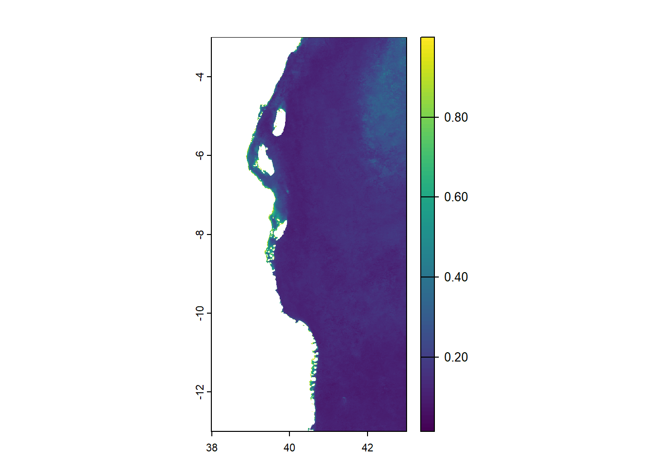
We will use satellite chlorophyll-a data measured by the MODIS sensor in Network Common Data Form (NetCDF) with file extension .nc for Tanzania coastal waters. The data will be loaded using rast() function of terra package (Hijmans, 2024).
class       : SpatRaster
dimensions  : 2224, 1112, 3  (nrow, ncol, nlyr)
resolution  : 0.004496807, 0.004496807  (x, y)
extent      : 37.99775, 42.9982, -12.99775, -2.996853  (xmin, xmax, ymin, ymax)
coord. ref. : lon/lat WGS 84
sources     : M2012214-2012244.vw.all_products.MYO.median.01aug12-31aug12.1368530332.data.nc:l2_flags
              M2012214-2012244.vw.all_products.MYO.median.01aug12-31aug12.1368530332.data.nc:chl_oc3
              M2012214-2012244.vw.all_products.MYO.median.01aug12-31aug12.1368530332.data.nc:land_mask
varnames    : l2_flags
              chl_oc3 (Chlorophyll-a concentration in sea water as measured by the MODIS sensor)
              land_mask
names       : l2_flags,       chl_oc3, land_mask
unit        :         , milligram m-3,
Our chl data is in SpatRaster with 2224 number of rows, 1112 number of columns and 3 number of layers. Layers include l2_flags, chl_oc3 and land_mask. The spatial resolution of our data is 0.004496807 pixels which is equivalent to 0.4946488 km approximately 0.5 km. We will select (using select() of tidyterra package) and plot (using plot() of terra package) the second layer (chl_oc3) which contain chlorophyll-a values.
Defining the extent
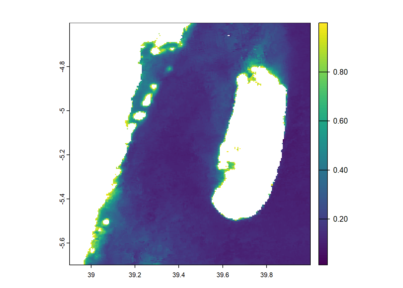
Suppose our analysis is focus only to a portion of Tanzania coastal area and not the whole area. So we need to crop that area on interest and leave the others. The focus of this post is around the Pemba Channel within longitude 38.9 and 40 East, and latitude -5.7, -4.6 South of the Equator. The first step is to specify the extent of our area using the ext() function of terra package (Hijmans, 2024):
Cropping
Then, we will crop our extent area from chl data using the crop() function of terra package (Hijmans, 2024).
Plotting the cropped area
Lastly we will plot our cropped area and visualize them;
We may also visualize the cropped area using leaflet package (Cheng et al., 2024);
pal = colorNumeric(c("#7f007f", "#0000ff",  "#007fff", "#00ffff", "#00bf00", "#7fdf00", "#ffff00", "#ff7f00", "#ff3f00", "#ff0000", "#bf0000"),  na.color = "transparent", values(site.crop |> select(chl_oc3) |> filter(chl_oc3 < 1)))

leaflet::leaflet() |>
  leaflet::addTiles() |>
  leaflet::addRasterImage(site.crop |> select(chl_oc3) |> filter(chl_oc3 < 1),
                          colors = pal,
                          opacity = 1) |>
  leaflet::addLegend(pal = pal,
                     values = values(site.crop |> select(chl_oc3) |> filter(chl_oc3 < 1)),
                     title = "Chlorophyll")
Thank you for following and do not miss the next post!!